Bandpass integration
The get_emission method implemented by any subclass of Model, including Sky, allows a numpy array of frequencies instead of a single frequency value to define a tophat bandpass and optionally a weights array of the same length to define a custom weight. PySM normalizes the weights array to unit integral then generates the emission at each of the specified frequencies, it multiplies it by the corresponding weight, and integrates them with the Trapezoidal rule. Instead of
having generating all the maps as PySM 2, PySM 3 keeps in memory just 1 array for the output map and then creates the maps at a specific frequency one at a time and accomulates it properly into the output array.
Integration and weighting is always performed in spectral radiance units \(Jy/sr\) and the weights are assumed to be given in those units, this is the same convention used by Planck HFI. For example if input templates are in \(K_{RJ}\) and the output is requested in \({K_{CMB}}\):
Each component
Modelloads the inputs from disk in \(K_{RJ}\)Evaluates the emission of the component at each of the frequency point
It weights them with bandpass weights that also include the transformation to spectral radiance units (this is performed by
utils.normalize_bandpass)Emission is accumulated into the output map and integrated in Spectral Radiance units
The integrated map is then converted back to \(K_{RJ}\) (thanks to the common factor applied also by
utils.normalize_bandpass). The output of eachModelobject is in \(K_{RJ}\) for compatibility with PySM 2.Finally the
Skyobject sums all the components and converts the output from \(K_{RJ}\) to the desired output unit, e.g. \(K_{CMB}\), using a factor computed byutils.bandpass_unit_conversion.
[2]:
sky = pysm3.Sky(nside=128, preset_strings=["d1", "s1"])
[3]:
map_100GHz_delta = sky.get_emission(100 * u.GHz)
[4]:
bandpass_frequencies = np.linspace(95, 105, 11) * u.GHz
[5]:
bandpass_frequencies
[5]:
[6]:
map_100GHz_tophat = sky.get_emission(bandpass_frequencies)
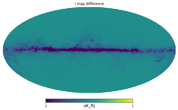
[7]:
hp.mollview(map_100GHz_delta[0] - map_100GHz_tophat[0], min=-1, max=1, title="I map difference", unit=map_100GHz_tophat.unit)
[8]:
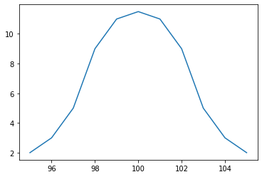
bandpass_weights = np.array([2,3,5,9,11,11.5,11,9,5,3,2])
[9]:
plt.plot(bandpass_frequencies,bandpass_weights);
[10]:
map_100GHz_bandpass = sky.get_emission(bandpass_frequencies, bandpass_weights)
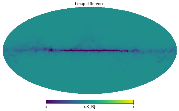
[11]:
hp.mollview(map_100GHz_bandpass[0] - map_100GHz_tophat[0], min=-1, max=1, title="I map difference", unit=map_100GHz_tophat.unit)
[ ]: