Reproduce PySM 2 small scales for dust polarization
The purpose of this notebook is to reproduce the analysis described in the PySM 2 paper to prepare the input templates used in the Galactic dust and synchrotron models. In summary we take input template maps from Planck or other sources, smooth them to remove noise and add small scale gaussian fluctuations.
[1]:
import os
os.environ["OMP_NUM_THREADS"] = "64"
[2]:
import os
import healpy as hp
import matplotlib.pyplot as plt
import numpy as np
from astropy.io import fits
%matplotlib inline
[3]:
hp.disable_warnings()
[4]:
plt.style.use("seaborn-talk")
[5]:
import pysm3 as pysm
import pysm3.units as u
[6]:
nside = 1024
lmax = 3 * nside - 1
Masks
Using the Planck 80% Galactic mask (the WMAP ones is for synchrotron).
The Planck foreground mask is also available with apodization of 2 or 5 degrees, here is the one with no apodization
[7]:
planck_map_filename = "HFI_Mask_GalPlane-apo0_2048_R2.00.fits"
[8]:
if not os.path.exists(planck_map_filename):
    !wget https://irsa.ipac.caltech.edu/data/Planck/release_2/ancillary-data/masks/$planck_map_filename
[9]:
fits.open(planck_map_filename)[1].header
[9]:
XTENSION= 'BINTABLE'           /Written by IDL:  Tue Dec  9 16:45:44 2014
BITPIX  =                    8 /
NAXIS   =                    2 /Binary table
NAXIS1  =                    8 /Number of bytes per row
NAXIS2  =             50331648 /Number of rows
PCOUNT  =                    0 /Random parameter count
GCOUNT  =                    1 /Group count
TFIELDS =                    8 /Number of columns
COMMENT
COMMENT  *** End of mandatory fields ***
COMMENT
EXTVER  =                    1 /Extension version
DATE    = '2014-12-09'         /Creation date
COMMENT
COMMENT  *** Column names ***
COMMENT
TTYPE1  = 'GAL020  '           / 20% sky coverage
TTYPE2  = 'GAL040  '           / 40% sky coverage
TTYPE3  = 'GAL060  '           / 60% sky coverage
TTYPE4  = 'GAL070  '           / 70% sky coverage
TTYPE5  = 'GAL080  '           / 80% sky coverage
TTYPE6  = 'GAL090  '           / 90% sky coverage
TTYPE7  = 'GAL097  '           / 97% sky coverage
TTYPE8  = 'GAL099  '           / 99% sky coverage
COMMENT
COMMENT  *** Column formats ***
COMMENT
TFORM1  = 'B       '           /
TFORM2  = 'B       '           /
TFORM3  = 'B       '           /
TFORM4  = 'B       '           /
TFORM5  = 'B       '           /
TFORM6  = 'B       '           /
TFORM7  = 'B       '           /
TFORM8  = 'B       '           /
COMMENT
COMMENT  *** Planck params ***
COMMENT
EXTNAME = 'GAL-MASK'           / Extension name
PIXTYPE = 'HEALPIX '           /
COORDSYS= 'GALACTIC'           / Coordinate system
ORDERING= 'NESTED  '           / Healpix ordering
NSIDE   =                 2048 / Healpix Nside
FIRSTPIX=                    0 / First pixel # (0 based)
LASTPIX =             50331647 / Last pixel # (0 based)
FILENAME= 'HFI_Mask_GalPlane-apo0_2048_R2.00.fits' / FITS filename
PROCVER = 'test    '           / Product version
COMMENT ------------------------------------------------------------------------
COMMENT Galactic emission masks, based on 353 GHz emission, apodized, and for
COMMENT various fractions of skycoverage. For general purpose usage.
COMMENT ------------------------------------------------------------------------
COMMENT For further details see Planck Explanatory Supplement at:
COMMENT   http://www.cosmos.esa.int/wikiSI/planckpla
COMMENT ------------------------------------------------------------------------
[10]:
planck_gal80_mask = hp.read_map(planck_map_filename, ("GAL080",))
[11]:
hp.mollview(planck_gal80_mask, title="Planck galactic mask 80% no apodization")
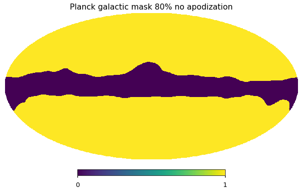
We need to downgrade the Planck mask from 2048 to 1024, so we average 4 pixels, we consider a pixel un-masked if 3 of the 4 pixels are unmasked.
[12]:
# total_mask = np.logical_and(hp.ud_grade(wmap_mask, nside), hp.ud_grade(planck_gal80_mask, nside)>=.75)
We can check how many pixels have the value of 0,0.25,0.5,0.75,1
[13]:
np.bincount((4*hp.ud_grade(planck_gal80_mask, nside)).astype(np.int64))
[13]:
array([ 2511882, 3288, 1665, 3317, 10062760])
[14]:
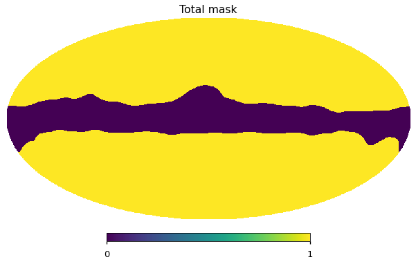
total_mask = hp.ud_grade(planck_gal80_mask, nside)>=.75
[15]:
hp.write_map("total_mask.fits", total_mask.astype(np.int), overwrite=True)
[16]:
hp.mollview(total_mask, title="Total mask")
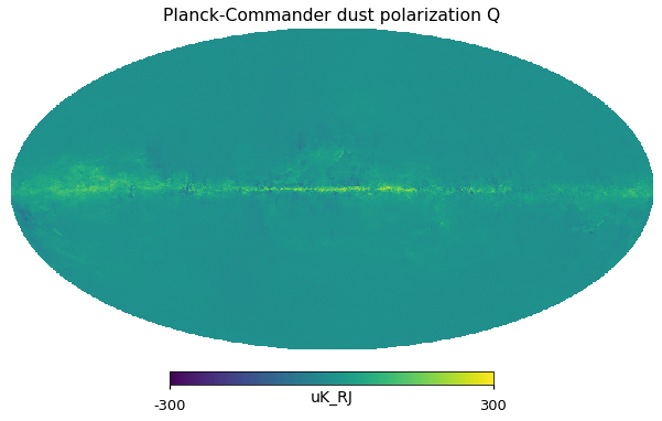
Download the dust polarization map from Planck / Commander
Download the dust polarization map from Commander, see:
We are trying to reproduce the PySM 2 results so we are using the Commander release 2 results. Later on we can switch to the last Planck release.
[17]:
commander_dust_map_filename = "COM_CompMap_DustPol-commander_1024_R2.00.fits"
[18]:
if not os.path.exists(commander_dust_map_filename):
    !wget https://irsa.ipac.caltech.edu/data/Planck/release_2/all-sky-maps/maps/component-maps/foregrounds/$commander_dust_map_filename
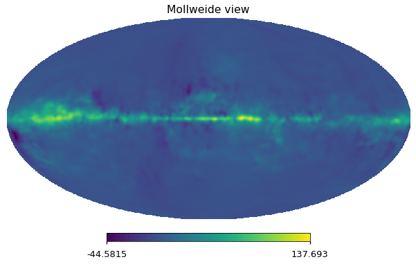
The input map has no temperature, we repeat the Q component for T as well, this doesn’t impact the polarization spectra:
[19]:
m_planck,h = hp.read_map("./COM_CompMap_DustPol-commander_1024_R2.00.fits", (0,0,1), h=True)
[20]:
h
[20]:
[('XTENSION', 'BINTABLE'),
 ('BITPIX', 8),
 ('NAXIS', 2),
 ('NAXIS1', 56),
 ('NAXIS2', 12582912),
 ('PCOUNT', 0),
 ('GCOUNT', 1),
 ('TFIELDS', 14),
 ('COMMENT', ''),
 ('COMMENT', ' *** End of mandatory fields ***'),
 ('COMMENT', ''),
 ('EXTNAME', 'COMP-MAP-DustPol'),
 ('EXTVER', 1),
 ('DATE', '2014-12-11'),
 ('COMMENT', ''),
 ('COMMENT', ' *** Column names ***'),
 ('COMMENT', ''),
 ('TTYPE1', 'Q_ML_FULL'),
 ('TTYPE2', 'U_ML_FULL'),
 ('TTYPE3', 'Q_ML_HM1'),
 ('TTYPE4', 'U_ML_HM1'),
 ('TTYPE5', 'Q_ML_HM2'),
 ('TTYPE6', 'U_ML_HM2'),
 ('TTYPE7', 'Q_ML_HR1'),
 ('TTYPE8', 'U_ML_HR1'),
 ('TTYPE9', 'Q_ML_HR2'),
 ('TTYPE10', 'U_ML_HR2'),
 ('TTYPE11', 'Q_ML_YR1'),
 ('TTYPE12', 'U_ML_YR1'),
 ('TTYPE13', 'Q_ML_YR2'),
 ('TTYPE14', 'U_ML_YR2'),
 ('COMMENT', ''),
 ('COMMENT', ' *** Column formats ***'),
 ('COMMENT', ''),
 ('TFORM1', 'E'),
 ('TFORM2', 'E'),
 ('TFORM3', 'E'),
 ('TFORM4', 'E'),
 ('TFORM5', 'E'),
 ('TFORM6', 'E'),
 ('TFORM7', 'E'),
 ('TFORM8', 'E'),
 ('TFORM9', 'E'),
 ('TFORM10', 'E'),
 ('TFORM11', 'E'),
 ('TFORM12', 'E'),
 ('TFORM13', 'E'),
 ('TFORM14', 'E'),
 ('COMMENT', ''),
 ('COMMENT', '*** Column units ***'),
 ('COMMENT', ''),
 ('TUNIT1', 'uK_RJ'),
 ('TUNIT2', 'uK_RJ'),
 ('TUNIT3', 'uK_RJ'),
 ('TUNIT4', 'uK_RJ'),
 ('TUNIT5', 'uK_RJ'),
 ('TUNIT6', 'uK_RJ'),
 ('TUNIT7', 'uK_RJ'),
 ('TUNIT8', 'uK_RJ'),
 ('TUNIT9', 'uK_RJ'),
 ('TUNIT10', 'uK_RJ'),
 ('TUNIT11', 'uK_RJ'),
 ('TUNIT12', 'uK_RJ'),
 ('TUNIT13', 'uK_RJ'),
 ('TUNIT14', 'uK_RJ'),
 ('COMMENT', ''),
 ('COMMENT', '*** Planck params ***'),
 ('COMMENT', ''),
 ('PIXTYPE', 'HEALPIX'),
 ('ORDERING', 'NESTED'),
 ('COORDSYS', 'GALACTIC'),
 ('POLCCONV', 'COSMO'),
 ('POLAR', 'True'),
 ('NSIDE', 1024),
 ('FIRSTPIX', 0),
 ('LASTPIX', 12582911),
 ('INDXSCHM', 'IMPLICIT'),
 ('BAD_DATA', -1.6375e+30),
 ('METHOD', 'COMMANDER'),
 ('AST-COMP', 'Dust-Polarization'),
 ('FWHM', 10.0),
 ('NU_REF', '353.0 GHz'),
 ('PROCVER', 'DX11D'),
 ('FILENAME', 'COM_CompMap_DustPol-commander_1024_R2.00.fits'),
 ('COMMENT', ''),
 ('COMMENT', '    Original Inputs'),
 ('COMMENT', '------------------------------------------------------------'),
 ('COMMENT', 'commander_dx11d2_pol_bpc_n1024_10arc_notempl_v1_full_dust.fits'),
 ('COMMENT', 'commander_dx11d2_pol_bpc_n1024_10arc_notempl_v1_hm1_dust.fits'),
 ('COMMENT', 'commander_dx11d2_pol_bpc_n1024_10arc_notempl_v1_hm2_dust.fits'),
 ('COMMENT', 'commander_dx11d2_pol_bpc_n1024_10arc_notempl_v1_hr1_dust.fits'),
 ('COMMENT', 'commander_dx11d2_pol_bpc_n1024_10arc_notempl_v1_hr2_dust.fits'),
 ('COMMENT', 'commander_dx11d2_pol_bpc_n1024_10arc_notempl_v1_yr1_dust.fits'),
 ('COMMENT', 'commander_dx11d2_pol_bpc_n1024_10arc_notempl_v1_yr2_dust.fits'),
 ('COMMENT', '------------------------------------------------------------'),
 ('COMMENT', 'For further details see Planck Explanatory Supplement at:'),
 ('COMMENT', ' http://www.cosmos.esa.int/wikiSI/planckpla'),
 ('COMMENT', '------------------------------------------------------------'),
 ('DATASUM', '2189663489'),
 ('CHECKSUM', 'ZAIMg2FMZ9FMf9FM')]
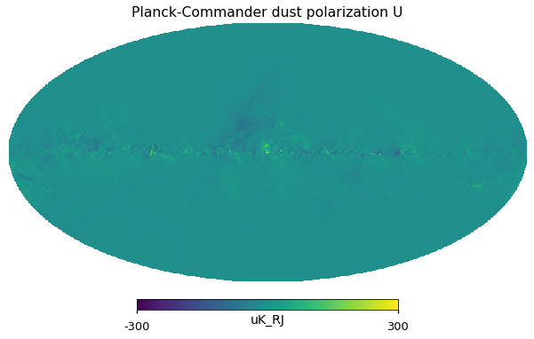
[21]:
for i_pol, pol in [(1, "Q"), (2, "U")]:
    hp.mollview(m_planck[i_pol], title="Planck-Commander dust polarization " + pol, unit="uK_RJ", min=-300, max=300)
[22]:
# A T map set to 0 is not supported by PolSpice
m_planck[0] = 1
Extend spectrum to small scales
Angular power spectrum with NaMaster
[23]:
import pymaster as nmt
[24]:
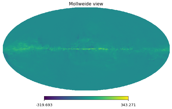
hp.mollview(m_planck[1])
[25]:
def run_namaster(m, mask):
    binning = nmt.NmtBin.from_nside_linear(hp.npix2nside(m.shape[-1]), 1)
    ell_arr = binning.get_effective_ells()
    ell_arr = np.concatenate([[0,0], ell_arr])
    f_2 = nmt.NmtField(mask, m.copy()) # namaster overwrites the map in place with the mask
    cl_22 = nmt.compute_full_master(f_2, f_2, binning)
    cl = np.zeros((3, len(ell_arr)), dtype=np.double)
    cl[1, 2:] = cl_22[0]
    cl[2, 2:] = cl_22[3]
    return ell_arr, cl
[ ]:
[26]:
ell_arr, spice_cl = run_namaster(m_planck[1:], total_mask)
[ ]:
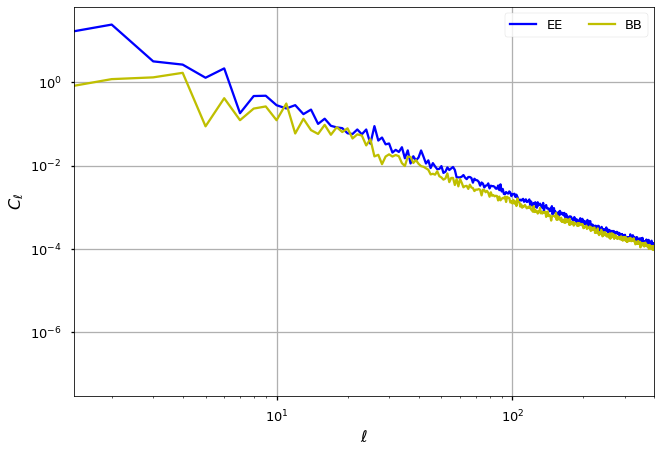
[28]:
plt.plot(ell_arr, spice_cl[1], 'b-', label='EE')
plt.plot(ell_arr, spice_cl[2], 'y-', label='BB')
plt.loglog()
plt.xlabel('$\\ell$', fontsize=16)
plt.ylabel('$C_\\ell$', fontsize=16)
plt.legend(loc='upper right', ncol=2, labelspacing=0.1)
plt.grid()
plt.xlim([0, 400])
plt.show()
/global/u2/z/zonca/condanamaster/lib/python3.7/site-packages/ipykernel_launcher.py:8: UserWarning: Attempted to set non-positive left xlim on a log-scaled axis.
Invalid limit will be ignored.
[29]:
ell = np.arange(spice_cl.shape[1])
cl_norm = ell*(ell+1)/np.pi/2
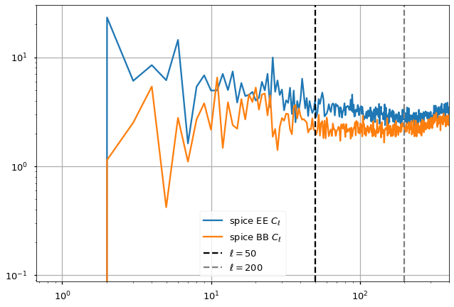
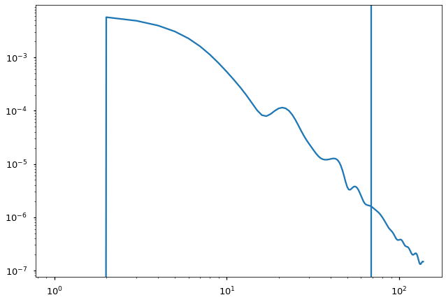
We plot the output power spectrum and also identify a range in \(\ell\) before white noise starts dominating and after the uncertainty at low-\(\ell\).
The power spectrum features a power law behaviour \(\ell < 200\) (linear in loglog axes), then white noise starts picking up until \(\ell=1000\) and then we see the smoothing applied to the maps (10 arcminutes).
[30]:
ell_fit_low = 50
ell_fit_high = 200
[31]:
plt.loglog(cl_norm * spice_cl[1], label="spice EE $C_\ell$")
plt.loglog(cl_norm * spice_cl[2], label="spice BB $C_\ell$")
plt.axvline(ell_fit_low, linestyle="--", color="black", label="$ \ell={} $".format(ell_fit_low))
plt.axvline(ell_fit_high, linestyle="--", color="gray", label="$ \ell={} $".format(ell_fit_high))
plt.legend()
plt.xlim([0, 400])
plt.grid();
/global/u2/z/zonca/condanamaster/lib/python3.7/site-packages/ipykernel_launcher.py:6: UserWarning: Attempted to set non-positive left xlim on a log-scaled axis.
Invalid limit will be ignored.
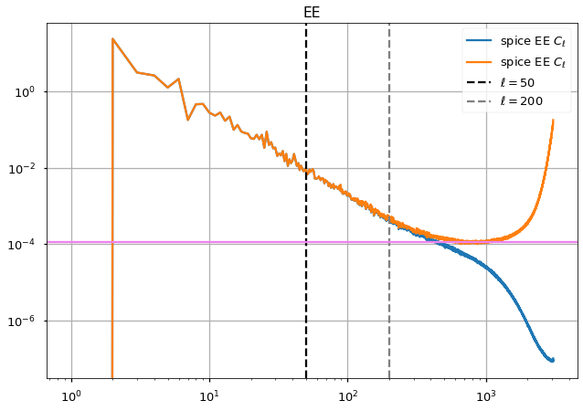
Fit noise bias
We want to fit for the high-ell slope so that we can extend that to higher ells, but the spectrum especially BB is dominated by noise, therefore we first fit an estimate of the noise at high ell and substract it out.
To do this we first “unsmooth” the map by the 10 arcmin beam used by Commander and then average where we see the spectrum flattening out. There are many parameters here we can tweak, the target here is just to check we can recover something similar to the PySM 2 paper.
[32]:
smoothing_beam = hp.gauss_beam(fwhm=(10 * u.arcmin).to_value(u.radian), lmax=lmax)
[33]:
noise_bias = (spice_cl[1:, 750:850] / smoothing_beam[750:850]**2).mean(axis=1)
[34]:
noise_bias = {"EE":noise_bias[0], "BB":noise_bias[1]}
[35]:
plt.title("EE")
plt.loglog(spice_cl[1], label="spice EE $C_\ell$")
#plt.loglog(spice_cl[2], label="spice BB $C_\ell$")
plt.loglog(spice_cl[1]/smoothing_beam**2, label="spice EE $C_\ell$")

plt.axvline(ell_fit_low, linestyle="--", color="black", label="$ \ell={} $".format(ell_fit_low))
plt.axvline(ell_fit_high, linestyle="--", color="gray", label="$ \ell={} $".format(ell_fit_high))
plt.legend()
for pol,color in zip(["EE", ], ["violet", ]):
    plt.axhline(noise_bias[pol], color=color, label=f"noise bias {pol}")
#plt.xlim([0, 400])
plt.grid();
[36]:
noise_bias
[36]:
{'EE': 0.00011287208896345207, 'BB': 0.00010224582025317983}
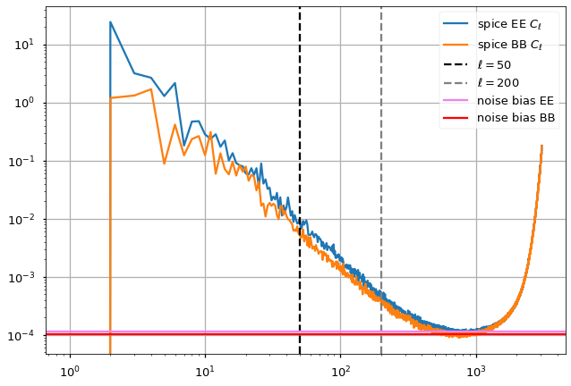
[37]:
plt.loglog(spice_cl[1]/smoothing_beam**2, label="spice EE $C_\ell$")
plt.loglog(spice_cl[2]/smoothing_beam**2, label="spice BB $C_\ell$")
plt.axvline(ell_fit_low, linestyle="--", color="black", label="$ \ell={} $".format(ell_fit_low))
plt.axvline(ell_fit_high, linestyle="--", color="gray", label="$ \ell={} $".format(ell_fit_high))
for pol,color in zip(["EE", "BB"], ["violet", "red"]):
    plt.axhline(noise_bias[pol], color=color, label=f"noise bias {pol}")
plt.legend()
plt.grid();
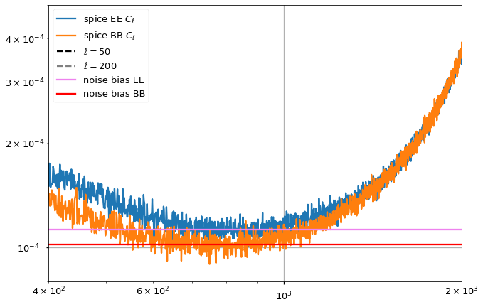
[38]:
plt.loglog(spice_cl[1]/smoothing_beam**2, label="spice EE $C_\ell$")
plt.loglog(spice_cl[2]/smoothing_beam**2, label="spice BB $C_\ell$")
plt.axvline(ell_fit_low, linestyle="--", color="black", label="$ \ell={} $".format(ell_fit_low))
plt.axvline(ell_fit_high, linestyle="--", color="gray", label="$ \ell={} $".format(ell_fit_high))
for pol,color in zip(["EE", "BB"], ["violet", "red"]):
    plt.axhline(noise_bias[pol], color=color, label=f"noise bias {pol}")
plt.legend()
plt.xlim([4e2, 2e3])
plt.ylim([8e-5, 5e-4])
plt.grid();
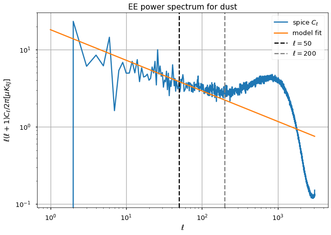
Fit for the slope at high ell
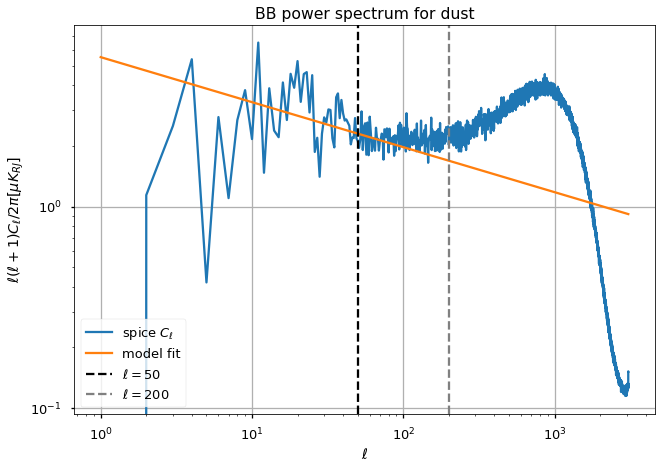
We assume the same model from the paper and fit for an amplitude and a power law exponent (slope in log-log)
[39]:
from scipy.optimize import curve_fit
[40]:
def model(ell, A, gamma):
    return A * ell ** gamma
[41]:
xdata = np.arange(ell_fit_low, ell_fit_high)
[42]:
A_fit, gamma_fit, A_fit_std, gamma_fit_std = {},{},{},{}
for pol,i_pol in [("EE",1),("BB",2)]:
    ydata = xdata*(xdata+1)/np.pi/2 * (spice_cl[i_pol][xdata] - noise_bias[pol])
    (A_fit[pol], gamma_fit[pol]), cov = curve_fit(model, xdata, ydata)

    A_fit_std[pol], gamma_fit_std[pol] = np.sqrt(np.diag(cov))
    plt.figure()
    plt.loglog(ell*(ell+1)/np.pi/2 * (spice_cl[i_pol] ), label="spice $C_\ell$")

    plt.loglog(A_fit[pol]*ell**gamma_fit[pol], label="model fit")
    plt.axvline(ell_fit_low, linestyle="--", color="black", label="$ \ell={} $".format(ell_fit_low))
    plt.axvline(ell_fit_high, linestyle="--", color="gray", label="$ \ell={} $".format(ell_fit_high))
    plt.legend()
    plt.grid()
    plt.ylabel("$\ell(\ell+1)C_\ell/2\pi [\mu K_{RJ}]$")
    plt.xlabel(("$\ell$"))

    plt.title(f"{pol} power spectrum for dust")
    #plt.xlim(0, 400)
    #plt.ylim(1, 30);
/global/u2/z/zonca/condanamaster/lib/python3.7/site-packages/ipykernel_launcher.py:10: RuntimeWarning: divide by zero encountered in power
  # Remove the CWD from sys.path while we load stuff.
/global/u2/z/zonca/condanamaster/lib/python3.7/site-packages/ipykernel_launcher.py:10: RuntimeWarning: divide by zero encountered in power
  # Remove the CWD from sys.path while we load stuff.
[43]:
A_fit, A_fit_std
[43]:
({'EE': 18.09672573027622, 'BB': 5.518135999977027},
 {'EE': 2.216649476829414, 'BB': 0.6670108771575787})
[44]:
gamma_fit, gamma_fit_std
[44]:
({'EE': -0.3957026535575404, 'BB': -0.22333811471731838},
 {'EE': 0.026341585170764382, 'BB': 0.025694460083852243})
The paper mentions a \(\gamma^{EE,dust} = -.31\) and a \(\gamma^{BB,dust} = -.15\).
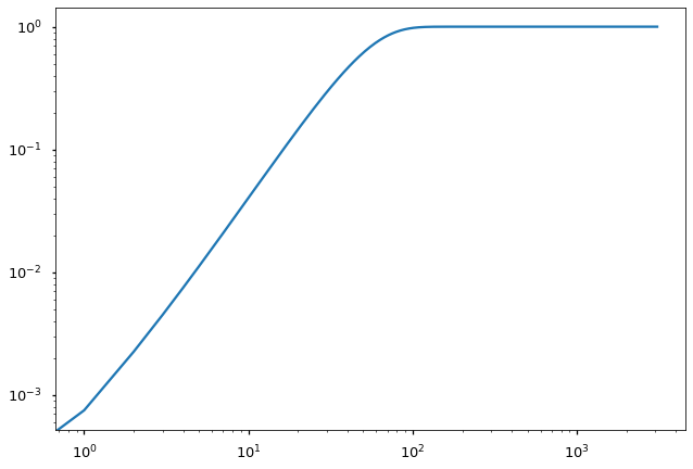
Window function
The window function is used to smooth the input templates to remove the high \(\ell\) noise and its inverse is used for the added small scales.
\(\ell_*^{dust}\)
[45]:
ell_star = 69
[46]:
theta_fwhm_deg = 180/ell_star
[47]:
theta_fwhm_deg
[47]:
2.608695652173913
[48]:
theta_fwhm = np.radians(theta_fwhm_deg)
[49]:
w_ell = hp.gauss_beam(fwhm=theta_fwhm, lmax=lmax)
[50]:
w_ell.shape
[50]:
(3072,)
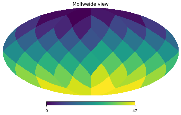
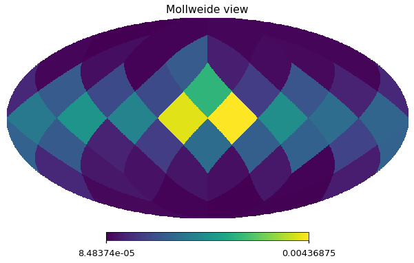
Process patches
This process doesn’t have a large impact on the output spectra, the idea is that in each \(N_{side}=2\) pixel we want to scale the gaussian fluctuations so that they are consistent with the power at low ell. So we will have higher gaussian fluctuations on the galaxy where there is stronger dust emission.
[51]:
patch_indices = hp.ud_grade(np.arange(hp.nside2npix(2)), nside)
[52]:
hp.mollview(patch_indices)
[53]:
zeros = np.zeros(len(ell), dtype=np.double)
[54]:
inv_w_ell = 1 - w_ell**2
[55]:
nside_patches = 2
n_patches = hp.nside2npix(nside_patches)
[56]:
plt.loglog(inv_w_ell)
[56]:
[<matplotlib.lines.Line2D at 0x2aace427a950>]
[57]:
hp.mollview(m_planck[1])

[58]:
m_sigma_G = hp.synfast([
    zeros,
    A_fit["EE"] * ell**gamma_fit["EE"] * inv_w_ell / cl_norm,A_fit["BB"] * ell**gamma_fit["BB"] * inv_w_ell / cl_norm,
    zeros, zeros, zeros], nside, new=True)
/global/u2/z/zonca/condanamaster/lib/python3.7/site-packages/ipykernel_launcher.py:3: RuntimeWarning: divide by zero encountered in power
  This is separate from the ipykernel package so we can avoid doing imports until
/global/u2/z/zonca/condanamaster/lib/python3.7/site-packages/ipykernel_launcher.py:3: RuntimeWarning: invalid value encountered in multiply
  This is separate from the ipykernel package so we can avoid doing imports until
[59]:
hp.mollview(m_sigma_G[0])
[60]:
N = {i_pol:np.zeros(n_patches, dtype=np.double) for i_pol in [1,2]}
[61]:
m_planck[0] = 0
[62]:
m_planck_smoothed = hp.alm2map(hp.smoothalm(hp.map2alm(m_planck, use_pixel_weights=True), fwhm=theta_fwhm),
                               nside=nside)
[63]:
hp.mollview(m_planck_smoothed[1])
[64]:
for i_patch in range(n_patches):
    print(i_patch)
    m_patch = np.zeros_like(m_planck_smoothed)
    m_patch[1:, patch_indices == i_patch] = m_planck_smoothed[1:, patch_indices == i_patch]
    cl_patch = hp.anafast(m_patch, lmax=2*ell_star, use_pixel_weights=True)
    for pol,i_pol in [("EE", 1),("BB",2)]:
        N[i_pol][i_patch] = np.sqrt(cl_patch[i_pol][ell_star] / n_patches / (A_fit[pol] * ell_star ** gamma_fit[pol]))
0
1
2
3
4
5
6
7
8
9
10
11
12
13
14
15
16
17
18
19
20
21
22
23
24
25
26
27
28
29
30
31
32
33
34
35
36
37
38
39
40
41
42
43
44
45
46
47
[65]:
plt.loglog(cl_patch[1])
plt.axvline(ell_star)
[65]:
<matplotlib.lines.Line2D at 0x2aacdc39aa50>
[66]:
hp.mollview(N[1])
[67]:
m_zeros = np.zeros(hp.nside2npix(nside), dtype=np.double)
[68]:
N_smoothed = hp.smoothing([m_zeros, hp.ud_grade(N[1], nside), hp.ud_grade(N[2], nside)], fwhm=np.radians(10))
[69]:
N_smoothed[1] /= N_smoothed[1].mean()
[70]:
N_smoothed[2] /= N_smoothed[2].mean()
[71]:
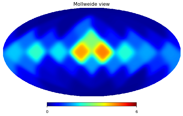
hp.mollview(N_smoothed[1], cmap="jet")
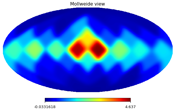
This also is quite different from Figure 9 in the paper, but it is not the main issue, possibly I need to use PolSpice instead of anafast?
[72]:
hp.mollview(N_smoothed[1], min=0, max=6, cmap="jet")
Run PolSpice on the total map and just on the small scales
Always using the same Gal80 Planck mask
[73]:
m_total = m_planck_smoothed + m_sigma_G * N_smoothed
[74]:
m_total[0] = 1
[75]:
_, cl_total = run_namaster(m_total[1:], total_mask)
[76]:
m_sigma_G[0]=1
[77]:
N_smoothed[0]=1
[78]:
_, cl_sigma_G_uniform = run_namaster(m_sigma_G[1:], total_mask)
Download PySM 2 templates
[79]:
for comp in "tqu":
    filename = f"dust_{comp}_new.fits"
    if not os.path.exists(filename):
        !wget https://portal.nersc.gov/project/cmb/pysm-data/pysm_2/$filename
[80]:
total_mask.shape
[80]:
(12582912,)
[81]:
total_mask_512 = hp.ud_grade(total_mask, 512)>=.75
[82]:
m_pysm2 = np.array([hp.read_map(f"dust_{comp}_new.fits") for comp in "tqu"])
[83]:
ell_arr_512, cl_pysm2 = run_namaster(m_pysm2[1:], total_mask_512)
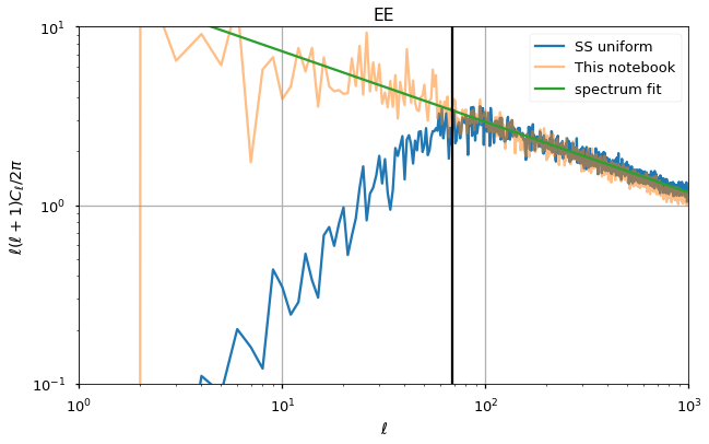
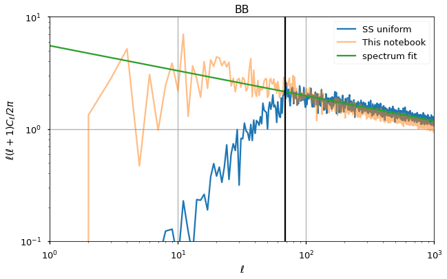
Check the impact of modifying the amplitude across the sky
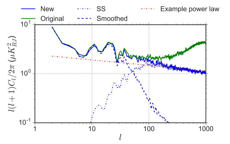
It has the effect of increasing how steeply the spectrum decreases at low-ell this has the same impact we can see on the plot in the paper copied at the bottom of the Notebook, the red line which is the fitted spectrum is less steep than the actual small scale realization.
[84]:
for pol, i_pol in [("EE",1),("BB",2)]:
    plt.figure(figsize=(10,6))
    #plt.loglog(cl_norm[:cl_pysm2.shape[1]]*cl_pysm2[i_pol], label="pysm2")
    plt.loglog(cl_norm*cl_sigma_G_uniform[i_pol], label="SS uniform")
    plt.loglog(cl_norm*cl_total[i_pol], label="This notebook", alpha=.5)

    #plt.loglog(cl_norm*spice_cl[i_pol], label="original")

    plt.loglog(A_fit[pol] * ell**gamma_fit[pol], label="spectrum fit")
    plt.axvline(ell_star, color="black")
    plt.title(pol)
    plt.legend()
    plt.xlim([1,1000])
    plt.ylim([1e-1, 1e1])
    plt.ylabel("$\ell(\ell+1)C_\ell/2\pi$")
    plt.xlabel("$\ell$")
    plt.grid();
/global/u2/z/zonca/condanamaster/lib/python3.7/site-packages/ipykernel_launcher.py:9: RuntimeWarning: divide by zero encountered in power
  if __name__ == '__main__':
/global/u2/z/zonca/condanamaster/lib/python3.7/site-packages/ipykernel_launcher.py:9: RuntimeWarning: divide by zero encountered in power
  if __name__ == '__main__':
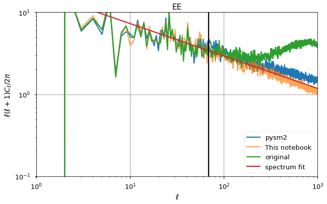
Compare PySM 2, the input and the output
[85]:
for pol, i_pol in [("EE",1),("BB",2)]:
    plt.figure(figsize=(10,6))
    plt.loglog(cl_norm[:cl_pysm2.shape[1]]*cl_pysm2[i_pol], label="pysm2")
    #plt.loglog(cl_norm*cl_sigma_G_uniform[i_pol], label="SS uniform")
    plt.loglog(cl_norm*cl_total[i_pol], label="This notebook", alpha=.7)

    plt.loglog(cl_norm*spice_cl[i_pol], label="original")

    plt.loglog(A_fit[pol] * ell**gamma_fit[pol], label="spectrum fit")
    plt.axvline(ell_star, color="black")
    plt.title(pol)
    plt.legend()
    plt.xlim([1,1000])
    plt.ylim([1e-1, 1e1])
    plt.ylabel("$\ell(\ell+1)C_\ell/2\pi$")
    plt.xlabel("$\ell$")
    plt.grid();
/global/u2/z/zonca/condanamaster/lib/python3.7/site-packages/ipykernel_launcher.py:9: RuntimeWarning: divide by zero encountered in power
  if __name__ == '__main__':
/global/u2/z/zonca/condanamaster/lib/python3.7/site-packages/ipykernel_launcher.py:9: RuntimeWarning: divide by zero encountered in power
  if __name__ == '__main__':
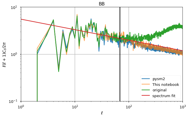
We can also compare with the dust BB plot (Figure 7) from the PySM 2 paper below
[86]:
from IPython.display import Image
Image("BB_dust_PySM_2_paper.png")
[86]: